Deep Learning from Scratch
读书笔记 Deep Learning from Scratch,Advanced Deep Learning with Python
数学的基本知识
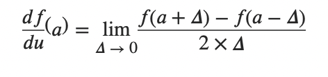
求导
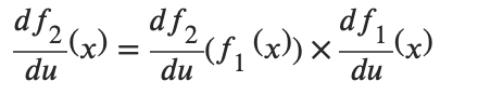
链式法则
例如:f(x) = sinx, g(x) = x^2^+1
f(g(x))' = sin(x^2^+1)'
f'(g(x))g'(x) = [sin(x^2^+1)]'* 2x
= 2cos(x^2^+1)x
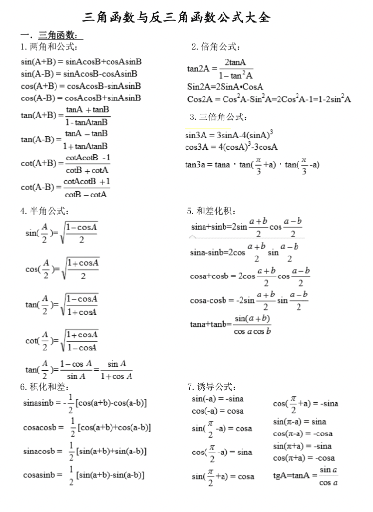
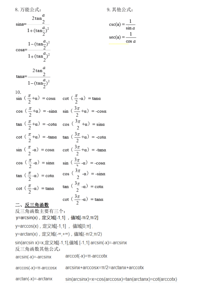
附上求导公式表:大一学的,已经忘光光了。
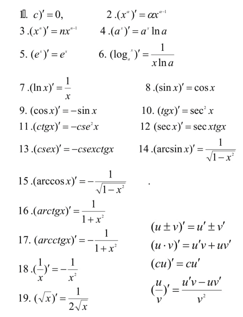
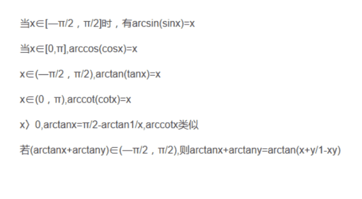
其中,反三角函数是给定比值,求对应的角度,而三角函数是给定角度,求比值。
tan是对边比邻边,
cot是邻边比对边,
sin是对边比斜边,
cos是邻边比斜边,
sec是1/cos 也就是斜边比邻边,
csc是1/sin 也就是斜边比对边。
哎,高中数学忘得精光……工作了虽然也用不到,但还是复习一下。
书里对链式法则的图解也很直观,两个delta相乘。
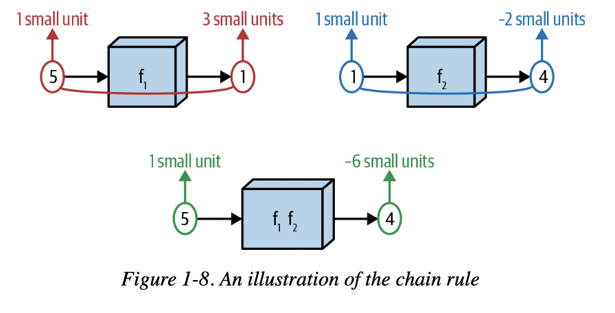
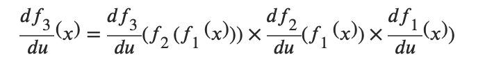
为什么要复习导数呢?因为,正向传播就是函数嵌套的过程,f~3~(f~2~(f~1~(x))),
而反向传播就是对这个嵌套函数进行递归求导。
向量乘法

概率
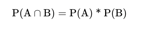

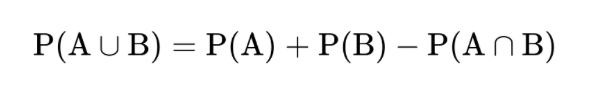
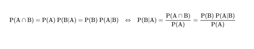
贝叶斯公式
Variance就是方差
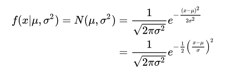
正态分布函数
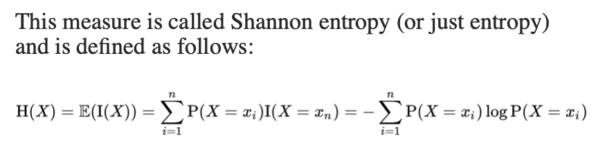
信息公式
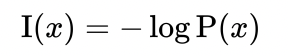
香农的信息熵:
偏导
一个多输入函数: (f(x,y))的正向和反向传播过程
(markdown里怎么打希腊字母:$\sigma$)
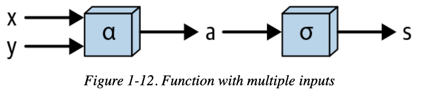
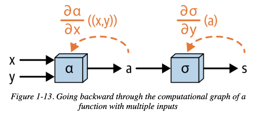
多输入函数对x求偏导:
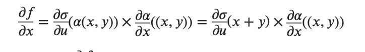
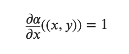
这个法则很重要,也很简单,它决定了反向传播最后一层(输入层)对某个变量的求导结果是多少。
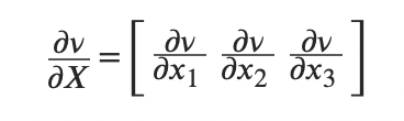
对向量求导:
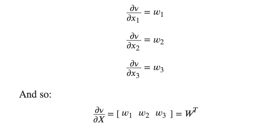
相当于对每个元素分别求导
Deep Learning:
“Repeatedly feed observations through the model, keeping track of the quantities computed along the way during this “forward pass.”
Calculate a loss representing how far off our model’s predictions were from the desired outputs or target.
Using the quantities computed on the forward pass and the chain rule math worked out in Chapter 1, compute how much each of the input parameters ultimately affects this loss.
Update the values of the parameters so that the loss will hopefully be reduced when the next set of observations is passed through the model.
每个Layer 都有Backward和Forward,也就是基本的Dense Layer
Normalize
其实这个很好理解,因为概率总是在0..1之间的。因此
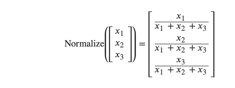
对向量的正则化就是把每个元素除以元素的总和。
Softmax函数
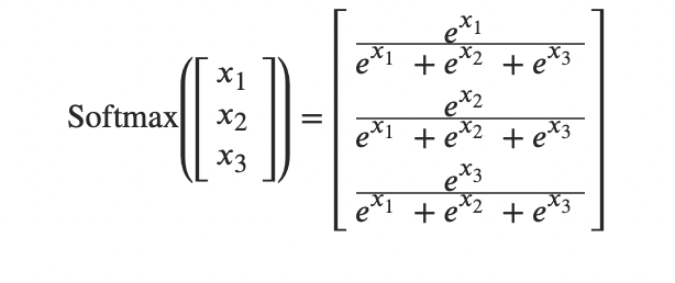
Softmax等于是更加突出了那个极值,放大了标准差。
Cross Entropy
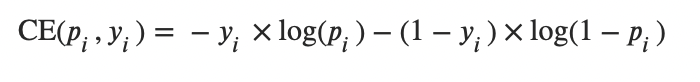
和前面的Softmax结合:

log消掉,剩下
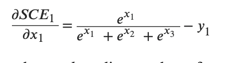
是不是很神奇!
所以SCE loss_grad 就等于 softmax_x -y
用ReLU取代Sigmoid来提升训练速度
Sigmoid的最大斜率是0.25,而且在<-2 或>2时,斜率接近0,这样导致更新变量的速度非常慢。
ReLU就是另一个极端,f(x) = x (x > 0) , 0 (x <= 0).
它也是符合激活函数的定义的,单调且非线性。
Leaky ReLU和Tanh
Tanh是长这样的,值域在(-1,1)
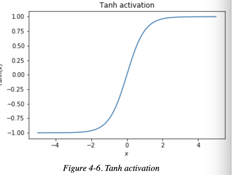
Leaky ReLU和ReLU不同的地方在 x < 0的地方,Leaky ReLU是y=kx,0 < k < 1.
此外,还有ReLU6等。
Momentum
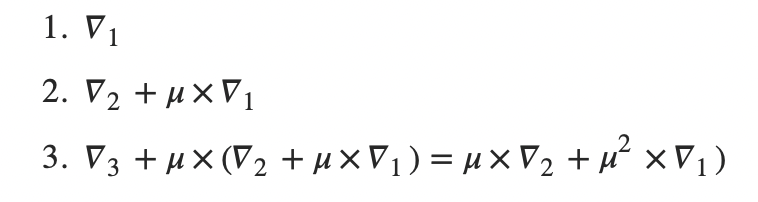
每一步更新x的速度不再是固定的,而是根据以往的速度计算得出。
Learning Rate Decay
随着Momentum慢慢变小,可能已经到了局部最优或者全局最优,再继续Training也只有很小的改变了。当Final Learning Rate低于阈值时,我们就可以停止训练了。
Weight Initialization
权重初始化,为什么需要这个呢?因为之前的Tanh,Sigmoid,在input = 0的时候有非常高的斜率。因此输入的权重 = 0并不是什么很好的选择。我们可以初始化权重,来让这种情况得到缓解。
Glorot初始化:

给每一层的权重赋值都是根据输入的个数和输出个数决定的。
Dropout
神经网络为啥不能无脑堆层数呢?因为容易过拟合,陷入局部最优。因此,我们不仅不能无脑堆,还要剪枝,把用不到的神经元关掉。很简单,把它们的权重设为0就好了,这样Forward和Backward都不会经过它。
同样,其他神经元的权重也会相应调整为Magnitude * (1-p)。
Convolutional
卷积核和矩阵,这个就不记录了,也是一样的矩阵元素相乘相加。
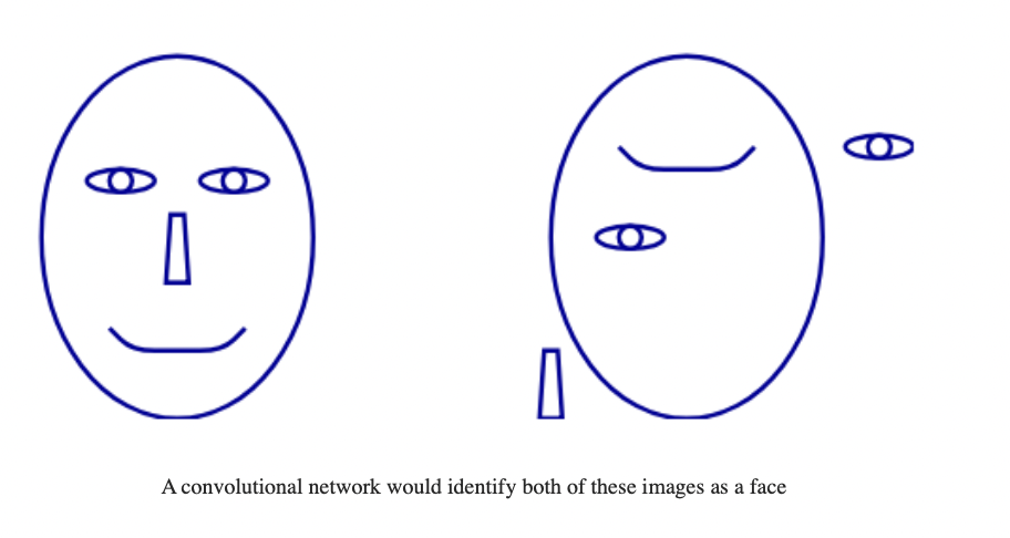
“The interpretation of each neuron of a fully connected layer is that it detects whether or not a particular combination of the features learned by the prior layer is present in the current observation.
The interpretation of a neuron of a convolutional layer is that it detects whether or not a particular combination of visual patterns learned by the prior layer is present at the given location of the input image.”
1x1卷积
可以改变输出的深度,也叫做Bottleneck layer
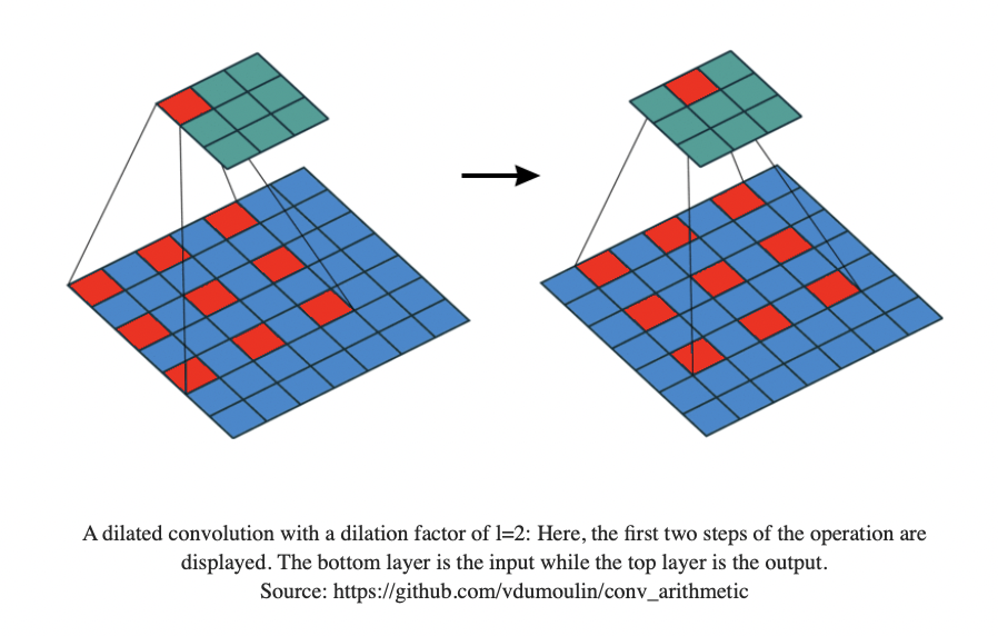
Dilated Convolution
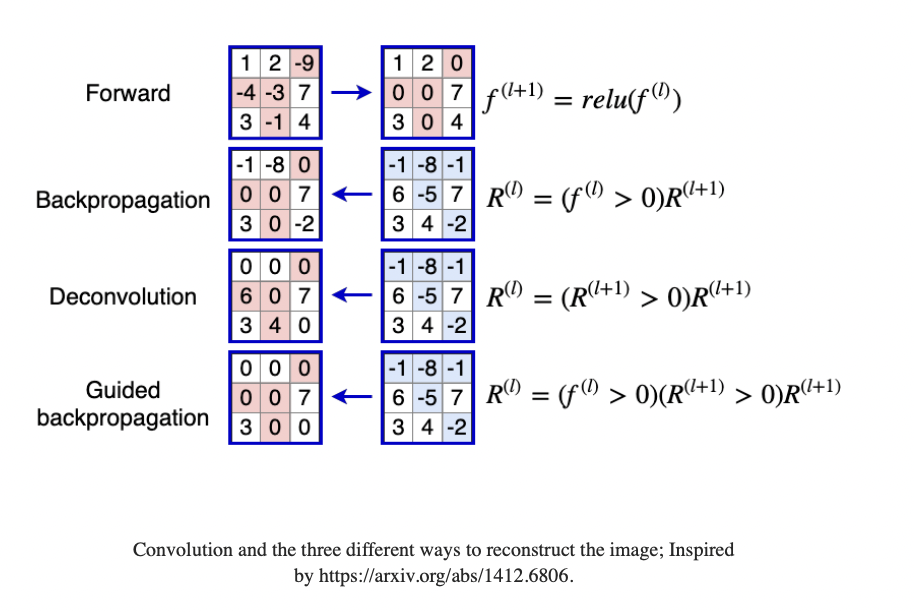
Guided back propagation
Flatten Layer
把m height width 的 matrix 变成 1 m height * width的vector
Pooling Layers
池化层,下采样,降分辨率
从ResNet开始,就很少会用到了,因为会损失信息
Padding
处理边缘值的时候,填充0。否则输出尺寸会比原来小。
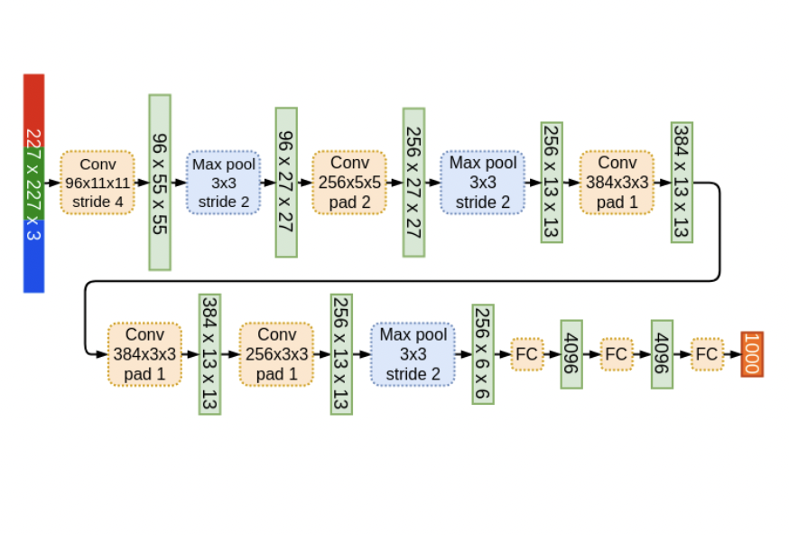
AlexNet
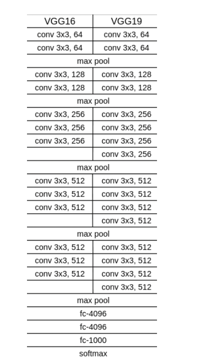
VGG
ResNet
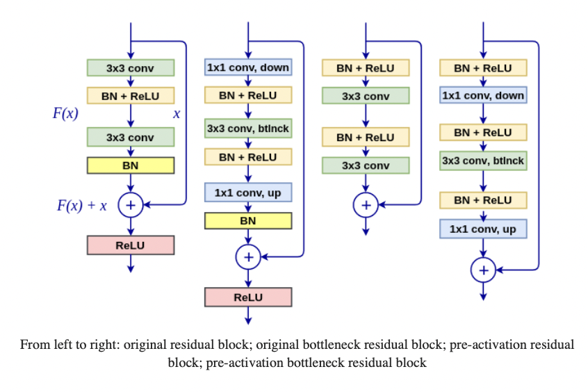
ResNet的作者发现,56层的神经网络比20层错误更多。理论上,更深的神经网络即使有很多不激活的神经元,也至少应该达到浅层网络同样的性能。
于是,残差网络诞生了,图中的四个都称为Residual Block(残差块),右边增加的这条路称为Identity Shourtcut Connection(Skip connection)。这样在正向传播的时候,不仅会传播Learned features,还会传播原始的输入信号,这样网络就可以决定跳过某些层。同时,也用了Padding来解决输出维度的问题。
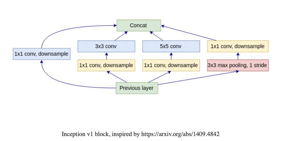
Inception
同一个物体,距离远在图片中就会小,而距离近则会更大。这对神经元产生了挑战,因为神经元的感受野大小是固定的。Inception从输入开始,就在各个Path上进行计算(Towers),每个Path包含不同大小、尺度的Filter等。
Inception V1
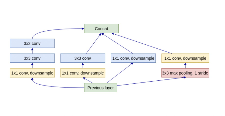
Inception V2 V3
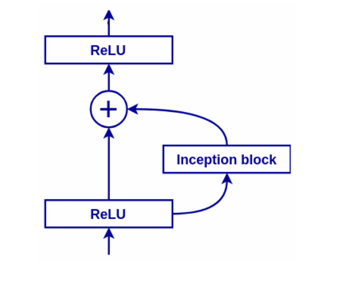
Inception V4(Inception Resnet)
Neural Architecture Search
让神经网络自行学习神经网络的参数:
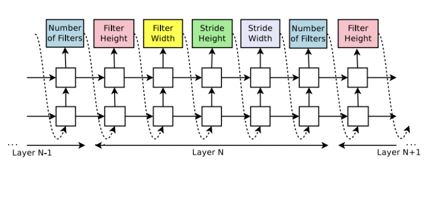
空白的block就是LSTM Cell
Picasso problem
Object Detection
Sliding window 滑动窗口
Two-stage:RPN(Region Proposal Network or RoI) 产生Bounding Box候选,供后续检测物体
YOLO
1、将图片分割成S*S的Cells
2、对每个Cell进行检测,输出0或多个检测出的物体
3、Intersection over Union(IoU)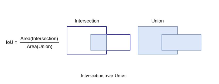
选出最大IoU的anchor box,能够代表物体的footprint
4、Non-maximum Suppression NMS 去除重复的bounding boxes
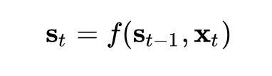
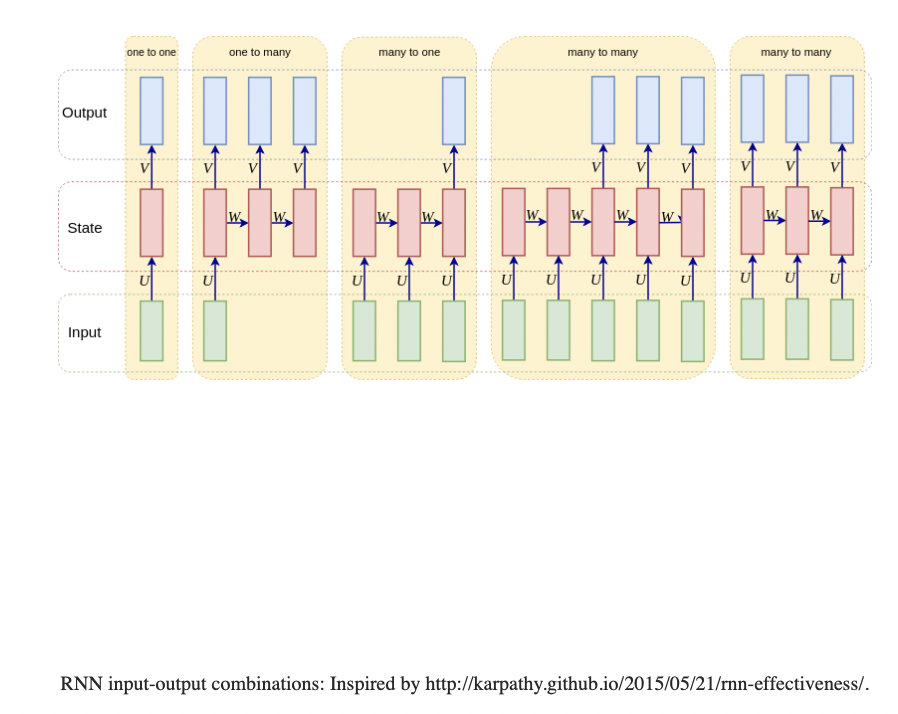
RNN
处理Sequence数据
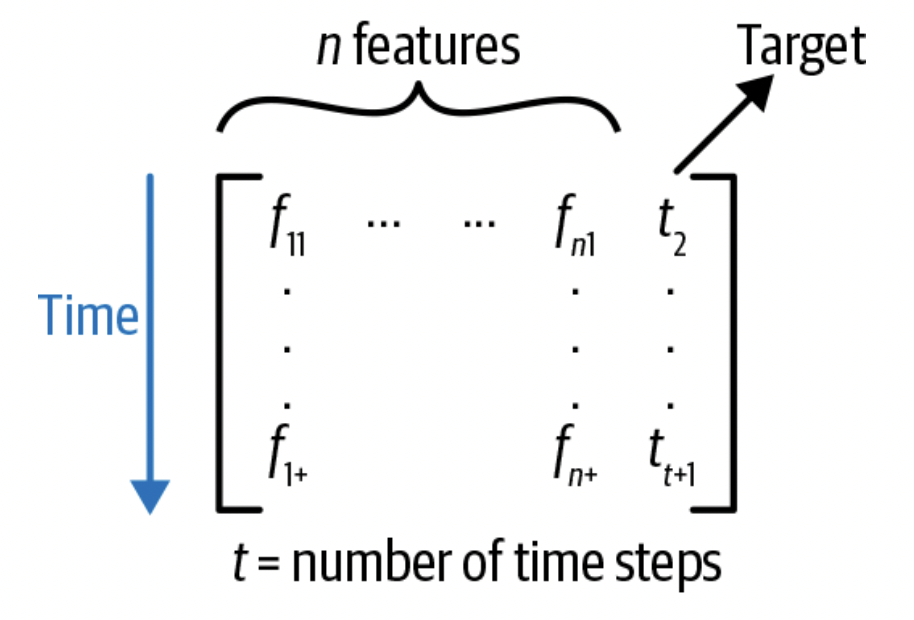
这样的原因在于,我们的输入是序列的数据,我们希望t=1的数据能影响到t=2的结果,而不是相互独立。我们希望把时间这个维度也加进来。
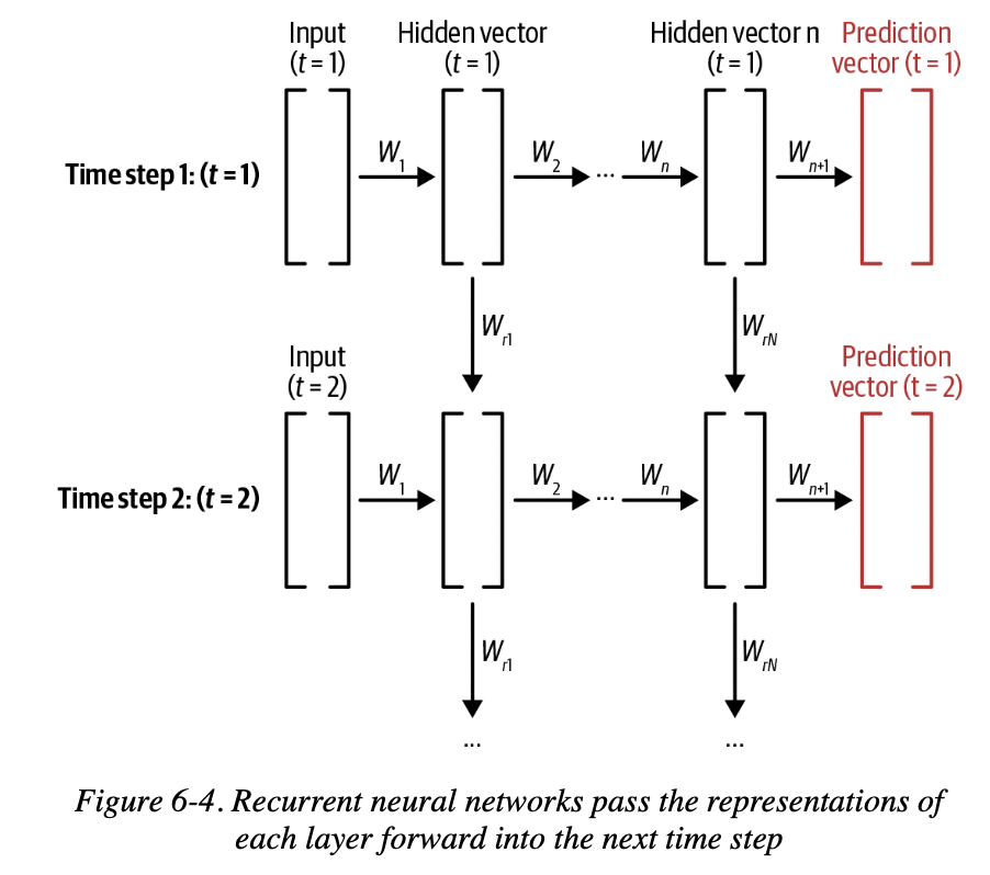
在t=1的时候,我们把随机初始化的向量输入,若干次迭代后得到一个输出向量。然后,我们把输出向量通过某种方式和下一次输入一起合并,得到t=2的输出,这样一直迭代下去。
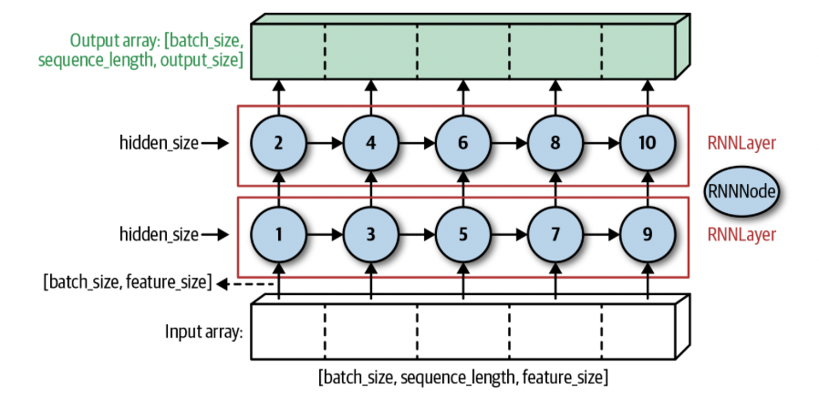
每一个RNN Layer都由固定数量的RNN Node组成。RNN的Back propagation会更新上一个time step的数值。
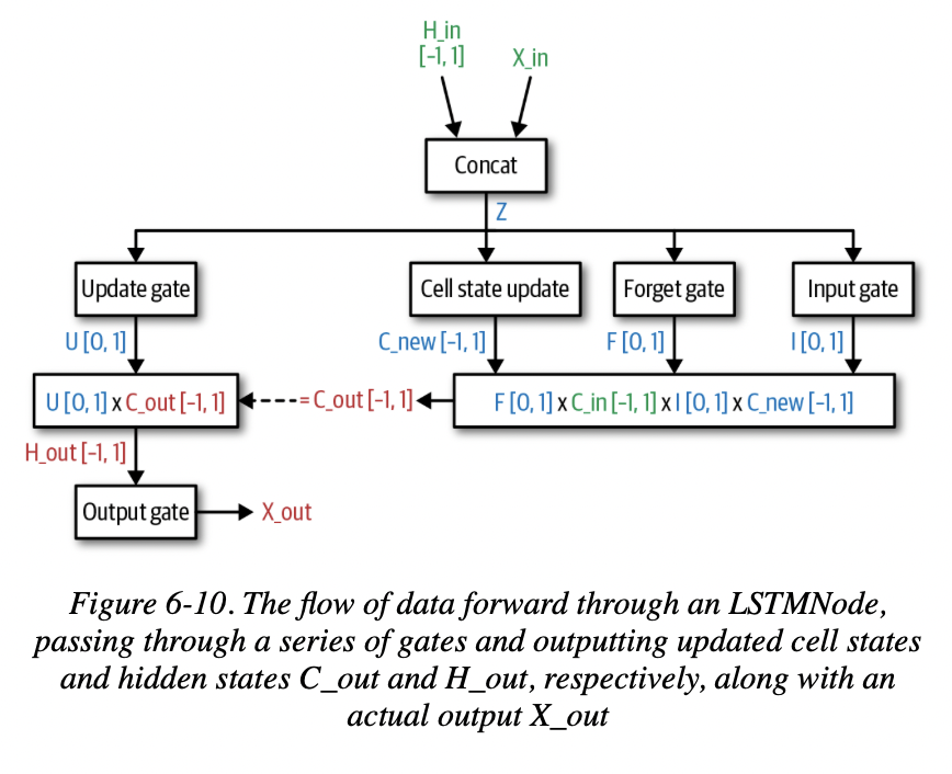
LSTM Node和Vanilla RNN Node的区别就在于它不仅仅存储了代表序列学习信息的Hidden Value,还存储了一个cell state,来建立Long Short term依赖关系。
Vanilla RNN的缺陷在于,它只能依赖最近的数据来预测未来,却难以拥有“记忆”,以及对久远数据的权重把握。
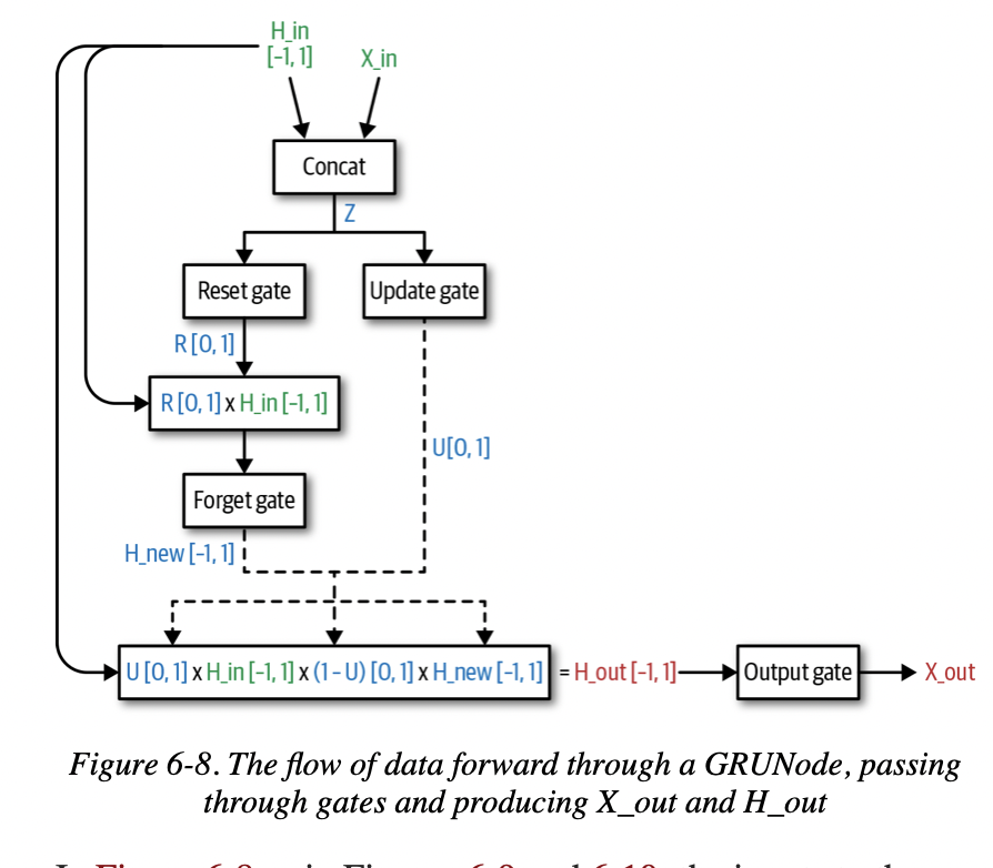
GRU Node
Learn to forget
LSTM Node
Transfer Learning
“TL is the process of applying an existing trained ML model to a new, but related, problem.”
U-Net
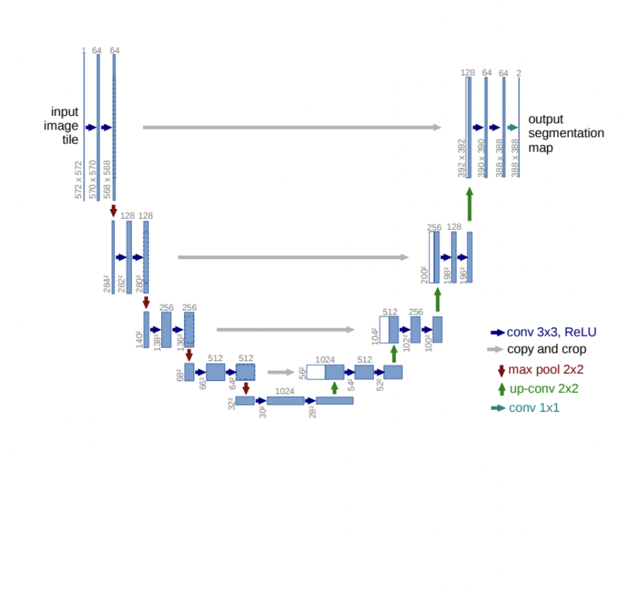
包含两部分,Encoder和Decoder
VAE
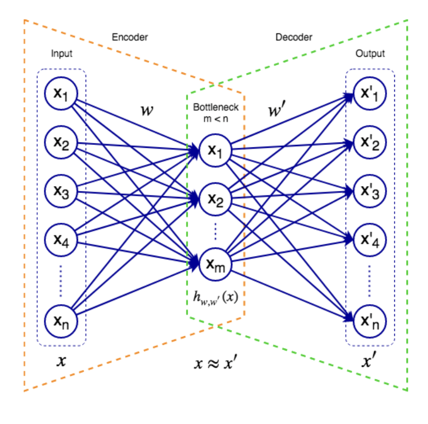
Encoder: 可以有多层hidden layer,将输入接收到网络中
Decoder: 试图从网络的内部feature重构输入
Denoising Autoencoder
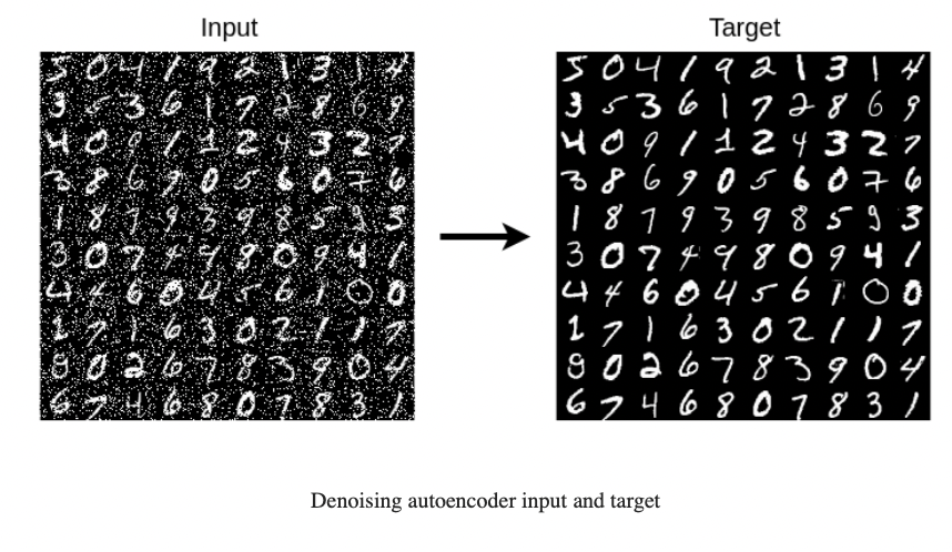
可以用这个Auto encoder来去噪
N-gram
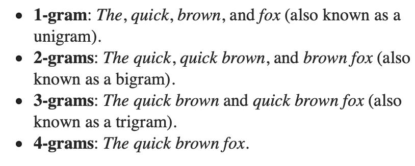
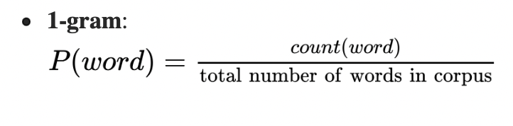
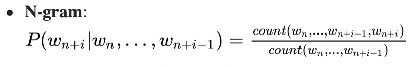
维度爆炸问题(curse of dimensionality):
n越大,可能性越大,复杂性指数升高
CBOW
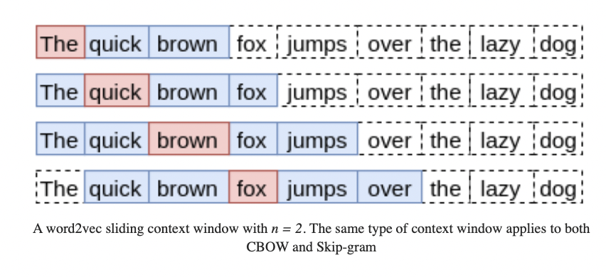
分辨出给定context哪个word是最可能出现的。
梯度消失和梯度爆炸
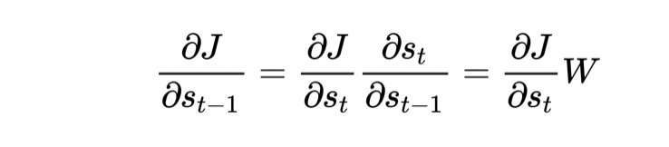
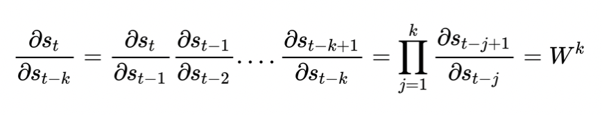
W > 1 就会发生梯度爆炸,W < 1 则会梯度消失
解决方法:LSTM
Forget Cell和Input Cell
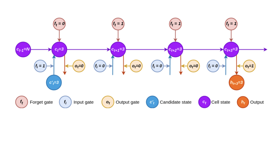
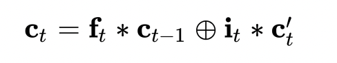
加号圆圈表示线性相加。
Seq2seq
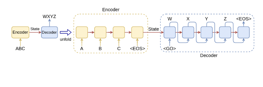
输入 A,B,C
输出W,X,Y,Z
encoder可以用任意RNN,论文里用的LSTM。
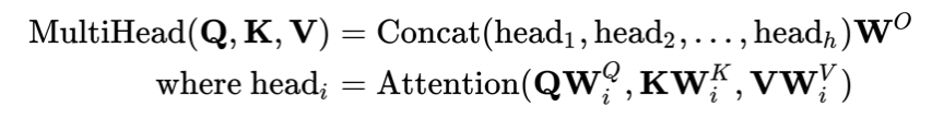
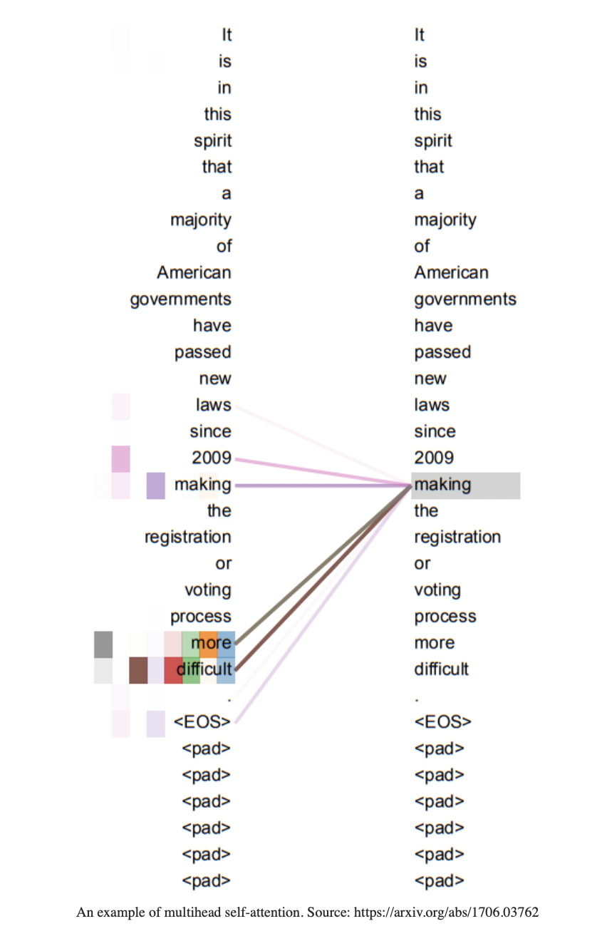
Transformer
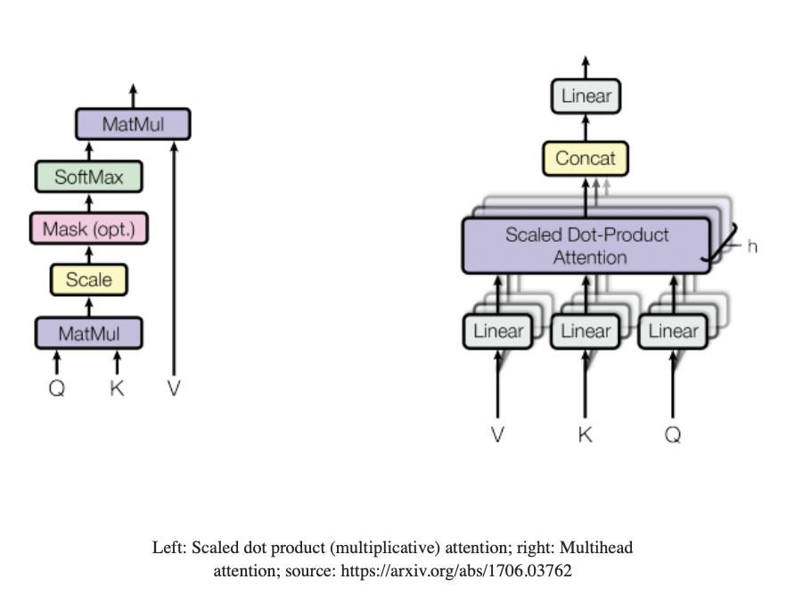
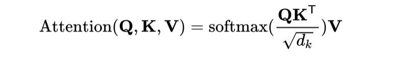
和数据库中的Query Key Value对应。
Transformer Model
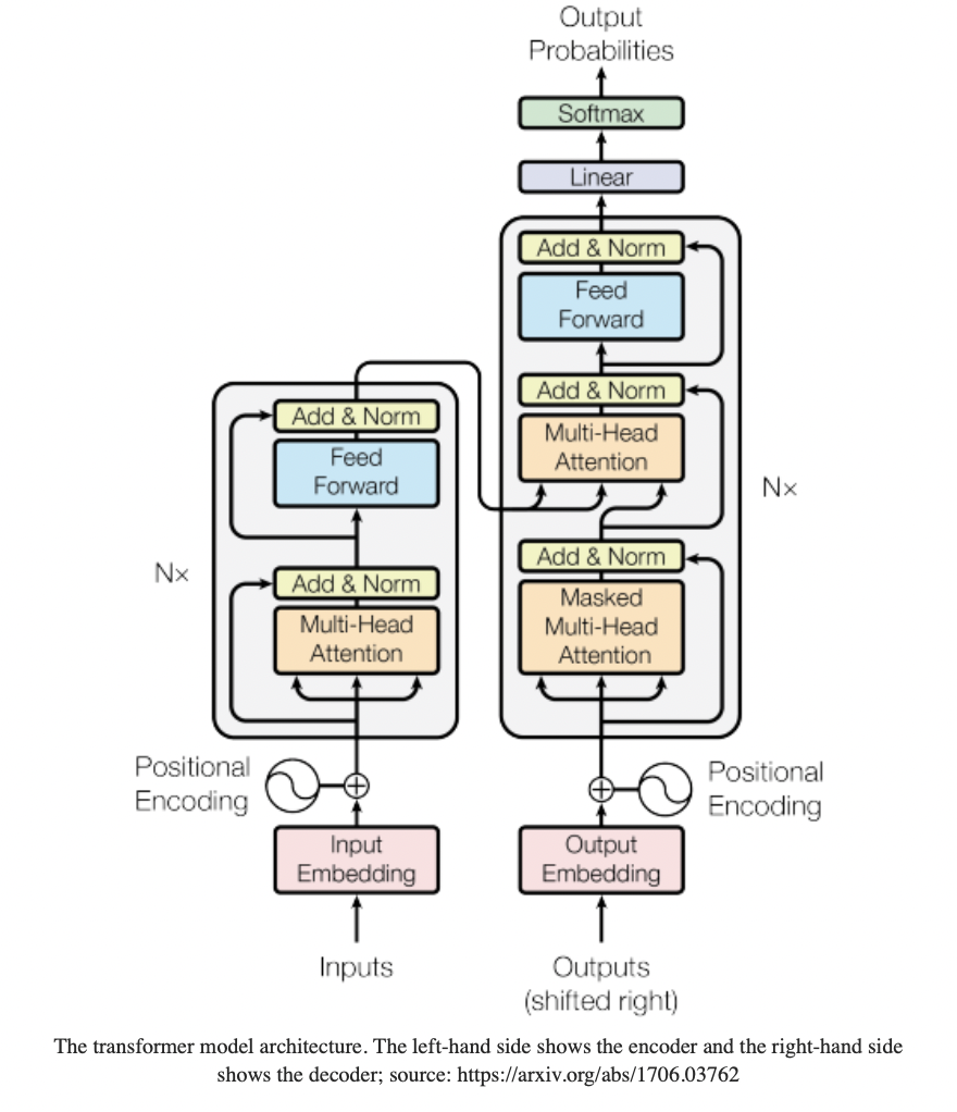
输入是one-hot encoded sequence
BERT
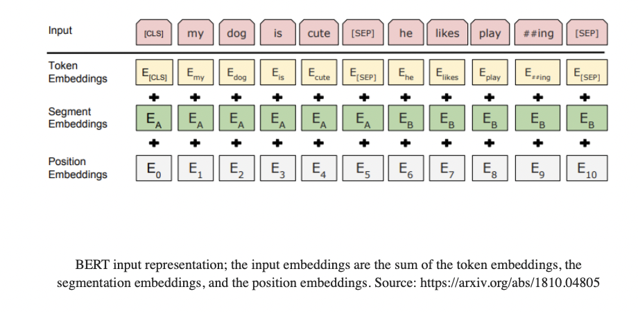
Masked Language Modeling(MLM)
80%的情况:把Word替换成MASK
“my dog is hairy → my dog is [MASK]”
10%的情况:替换成随机单词
“my dog is hairy → my dog is apple”
10%的情况:不变
“my dog is hairy → my dog is hairy”
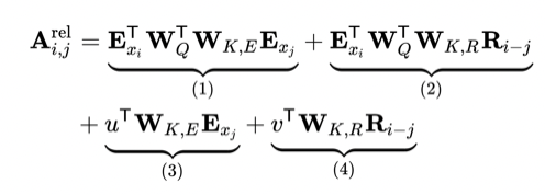
Transformer attention
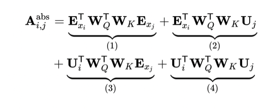
1 表示content based word i 和 word j 的关联性
2 表示 word i 和 pos j 上的关联性,比如 i 为cream,那么 j 为ice的可能性就很大
3 2的反面
4 pos i和pos j的关联性
Relative positional encodings
把绝对位置换成了相对位置